Subdivision spline curves

There is one more point of view on generation of B-spline curves. The subdivision rules for a degree M + 1 uniform B-spline curve (the Lane-Riesenfeld algorithm) are well known [1] and related to the binomial coefficients.

Start with a piecewise linear curve (the blue one below).
Insert new vertices at the midpoints (the splitting step)
P_2i⁰ = P_i, P_2i+1⁰ = (P_i + P_i+1)/2.
Average each vertex with the "next" neighbor M times (the averaging step)
P_i^k = (P_i^k-1 + P_i+1^k-1)/2, k = 1,...,M, (*)
where coefficients (1/2, 1/2) are called averaging mask.
Repeat splitting and averaging N times

Closed spline curves

Here the Lane-Riesenfeld algorithm is applied to a closed spline curve (i.e. P_N+1 = P₁). You can change control points of the curve and set new N, M values.

move
add
delete

N
M

The second B-spline is generated by the basis functions.

Modified subdivision algorithm

It is usefull to combine two averaging steps and rewrite (*) in symmetric form
P_i^k = (P_i-1^k-1 + 2 P_i^k-1 + P_i+1^k-1)/4,
with averaging mask (1/4, 1/2, 1/4). After one averaging (M = 1) we get the cubic B-spline. Now to get a curve with clamped endpoins we use this averaging mask for all points excluding endpoints. To get a curve with crease at a point we can just exclude the point from averagings.

move
add
delete

N
M

The limit point position and the tangent vector

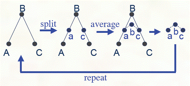
Consider the cubic B-spline subdivision operation for the ABC triangle (N = 1, M = 1 above). After one iteration we get similar abc triangle and can use the same operation ad infinitum to get the limit position of the B point.
limit

One can write this operation in the matrix form, compute its eigenvalues and eigenvectors and find the limit point position and the tangent vector without infinite subdivisions. E.g. the evaluation mask for the cubic B-spline is (1, 4, 1)/6. So we can add two more final steps to the subdivision rules (we will use them for spline surfaces later)

Use the evaluation mask and push the resulting points to the limit positions.
Compute the tangents using the tangent mask.

[1] Jos Stam On Subdivision Schemes Generalizing Uniform B-spline Surfaces of Arbitrary Degree Computer Aided Geometric Design. March 2001, 18. pp. 383-396.

Contents Previous: Cubic Bezier patch with adaptive subdivision Next: Loop subdivision spline surface
updated 25 Mar 2013